Precision、Recall、P-R曲线、ROC、AUC、mAP

1. Precision和Recall

对于二分类问题，可将样例根据其真实类别与学习器预测类别的组合划分为：

TP (True Positive)：预测为真，实际为真
FP (False Positive)：预测为真，实际为假
TN (True Negative)：预测为假，实际为假
FN (False Negative)：预测为假，实际为真

令 TP、FP、TN、FN分别表示其对应的样例数，则显然有 TP + FP + TN + FN = 样例总数
分类结果的 “混淆矩阵” 如下：

	实际为真 T	实际为假 F
预测为正例 P	TP (预测为1，实际为1)	FP (预测为1，实际为0)
预测为负例 N	FN (预测为0，实际为1)	TN (预测为0，实际为0)

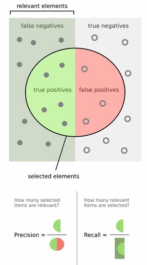
\[ （查准率）Precision = \frac{TP}{TP + FP} \\ \\ \\ {\color{Purple}{（预测的好瓜中有多少是真的好瓜）}} \]

\[ （查全率）Recall = \frac{TP}{TP + FN} \\ \\ {\color{Purple}{（所有真正的好瓜中有多少被真的挑出来了）}} \]

2. P-R曲线

一般来说，查准率高时，查全率往往偏低，而查全率高时，查准率往往偏低。通常只有在一些简单任务中，才可能使得查全率和查准率都很高。在很多情况，我们可以根据学习器的预测结果，得到对应预测的 confidence scores 得分(有多大的概率是正例)，按照得分对样例进行排序，排在前面的是学习器认为”最可能“是正例的样本，排在最后的则是学习器认为“最不可能”是正例的样本。每次选择当前第 \(i\) 个样例的得分作为阈值 \((1 \leq i \leq 样例个数)\)，计算当前预测的前 \(i\) 为正例的查全率和查准率。然后以查全率为横坐标，查准率为纵坐标作图，就得到了我们的查准率-查全率曲线: P-R曲线

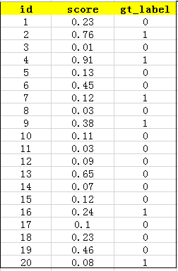
举例说明：以下摘自多标签图像分类任务的评价方法-mAP

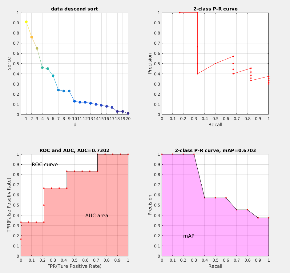
在一个识别图片是否是车，这样一个二分类任务中，我们训练好了一个模型。假设测试样例有20个，用训练好模型测试可以得到如下测试结果：其中 id (序号)，confidence score (置信度、得分) 和 ground truth label (类别标签)

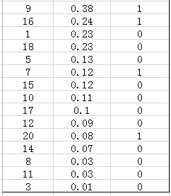
接下来对 confidence score 排序，得到：

然后我们开始计算P-R曲线值，将排序后的样例，从 \(i = 0\) 到 \(i = 20\) 遍历，每次将第 \(i\) 个样例的 confidence scores 做为阈值，前 \(i\) 个预测为正例时，计算对应的 Precision 和 Recall。

例如，当 \(i = 1\) 时，预测了一个做为正例，其余的都预测为反例，此时的阈值为 0.91。此时的 TP=1 就是指第4张，FP=0，FN=5 为第2、9、16、7、20 的图片，TN=15为13,19,6,1,18,5,15,10,17,12,14,8,11,3。Precision = TP/(TP+FP) = 1/(1+0) = 0 ；Recall = TP/(TP+FN) = 1/(1+5)=1/6 。接着计算当 \(i = 2\) 时，以此类推…

为了便于理解，我们再讲一个例子当 \(i = 5\) 时，表示我们选了前5个预测结果认为是正例（对应圆圈中的TP和FP），此时阈值为0.45，我们得到了 top-5 的结果如下：

在这个例子中，TP 就是指第4和第2张图片，FP 就是指第13，19，6张图片。方框内圆圈外的元素（FN和TN）是相对于方框内的元素而言，在这个例子中，是指 confidence score 小于当前阈值的元素，即：

3. ROC 与 AUC

ROC 全称是“受试者工作特征”（Receiver Operating Characteristic）。ROC 曲线的面积就是 AUC（Area Under the Curve）。AUC用于衡量“二分类问题”机器学习算法性能（泛化能力）。

思想：和计算 P-R 曲线方法基本一致，只是这里计算的是真正率(True Positive rate) 和假正率(False Positive rate)，以 FPR 为横轴，TPR 为纵轴，绘制的曲线就是 ROC 曲线，ROC 曲线下的面积，即为 AUC

\[ （真正率）TPR = \frac{TP}{TP + FN} \]

\[ （假正率）FPR = \frac{FP}{FP + TN} \]

4. mAP

接下来说说 AP 的计算，此处参考的是 PASCAL VOC CHALLENGE 的计算方法。首先按照 R-P曲线计算方式计算 Precision 和 Recall。然后设定一组阈值，[0, 0.1, 0.2, …, 1]，计算 Recall 大于第 \(i\) 个阈值的R-P集合中，对应的 Precision 的最大值。这样，我们就计算出了11个 Precision。mAP 即为这11个 Precision 的平均值。这种方法英文叫做 11-point interpolated average precision
相应的Precision-Recall曲线（这条曲线是单调递减的）如下：

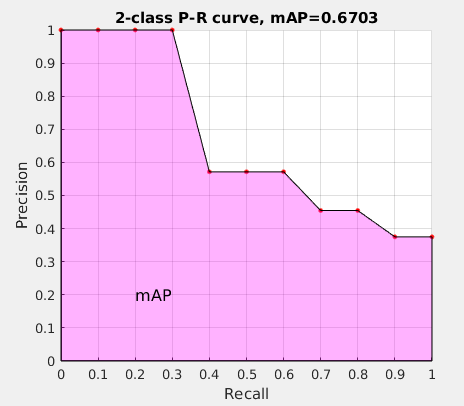
AP 衡量的是学出来的模型在每个类别上的好坏，mAP 衡量的是学出的模型在所有类别上的好坏，得到 AP 后 mAP 的计算就变得很简单了，就是取所有 AP 的平均值。

5. 代码简单实现

% Creation          :  25-Apr-2018 16:01
% Last Reversion    :  25-Apr-2018 16:25
% Author            :  Lingyong Smile {smilelingyong@163.com}
% File Type         :  Matlab
% -----------------------------------------------------------
% mAP_learning()
% This script is used to learning precesion, recall, RP curve, 
% ROC and AUC curve, and mAP.
% ------------------------------------------------------------
% Copyright (c) 2018, Lingyong Smile

%% Initialization
clc;
clear;
close all;
dbstop if error;

%% Load data
data = ...
[[1:20]', ...
[0;1;0;1;0;0;1;0;1;0;0;0;0;0;0;1;0;0;0;1], ...
[0.23; 0.76; 0.01; 0.91; 0.13; 0.45; 0.12; 0.03; 0.38; 0.11; 0.03; 0.09; 0.65; 0.07; 0.12; 0.24; 0.1; 0.23; 0.46; 0.08]];

%% Plot sorted data
[~, sort_idx] = sort(data(:,3), 'descend');
data = data(sort_idx, :);   % descend sort data of confident
figure(1);
subplot(2, 2, 1);
hold on;
% plot(data(:, 1), data(:, 3), '*r'); 
x = [1:length(data(:, 1))+1];
y = [data(:, 3); NaN];
c = y;
patch(x, y, c, 'EdgeColor','interp','Marker','o','MarkerFaceColor','flat'); % which is equals to the comment line
title('data descend sort');
xlabel('id');
ylabel('sorce');
set(gca, 'xtick', [1:size(data, 1)], 'ytick', [0:0.1:1]);  % set grid properties
grid on;

%% Calculate Precision and Recall, False positive rate and True positive rate
for i = 1:size(data, 1)
    TP = sum(data(1:i, 2) == 1);
    FP = sum(data(1:i, 2) == 0);
    FN = sum(data(i+1:end, 2) == 1);
    TN = sum(data(i+1:end, 2) == 0);
    Precision(i) = TP / (TP + FP);
    Recall(i) = TP / (TP + FN);
    TPR(i) = TP / (TP + FN);
    FPR(i) = FP / (FP + TN);
end

%% Plot P-R curve
subplot(2, 2, 2);
plot(Recall, Precision, '-r');
hold on;
plot(Recall, Precision, '.r', 'MarkerSize', 10, 'MarkerEdgeColor', 'r', 'MarkerFaceColor', 'r'); % plot point
set(gca,'xtick',[0:0.1:1], 'ytick', [0:0.1:1]); 
grid on;
axis([0, 1, 0, 1]);
title('2-class P-R curve');
xlabel('Recall');
ylabel('Precision');

%% Plot mAP
ap = [];
thresh = 0:0.1:1;
for t = thresh
    p = max(Precision(Recall >= t));
    if isempty(p)
        p = 0;
    end
    ap(end+1) = p;
end
mAP = sum(ap) / 11;

subplot(2, 2, 4);
hold on;
plot(thresh, ap, '-r');
plot(thresh, ap, '.r', 'MarkerSize', 10, 'MarkerEdgeColor', 'r', 'MarkerFaceColor', 'r'); % plot point
patch('Faces', 1:length(thresh)+2, 'Vertices', [[0, thresh, 1]', [0, ap, 0]'], 'FaceColor','magenta','FaceAlpha',.3);
text(0.2, 0.2, 'mAP', 'FontSize', 12);  % text the mAP
set(gca,'xtick',[0:0.1:1], 'ytick', [0:0.1:1]); 
grid on;
axis([0, 1, 0, 1]);
title(sprintf('2-class P-R curve, mAP=%.4f', mAP));
xlabel('Recall');
ylabel('Precision');

%% Plot ROC and AUC
ap = [];
thresh = [0:1/length(FPR):1];
for t = thresh
    p = max(TPR(FPR <= t));
    if isempty(p)
        p = 0;
    end
    ap(end+1) = p;
end
AUC = sum(ap) / length(thresh);

subplot(2, 2, 3);
hold on;
plot(FPR, TPR, '-.b');
plot(FPR, TPR, '.r', 'MarkerSize', 10, 'MarkerEdgeColor', 'r', 'MarkerFaceColor', 'r'); % plot point
% patch([0, FPR, 1], [0, TPR, 0], 'r'); % which is simple fill red color 
patch('Faces', 1:length(FPR)+2, 'Vertices', [[0, FPR, 1]', [0, TPR, 0]'], 'FaceColor','red','FaceAlpha',.3);
text(0.1, 0.9, 'ROC curve', 'FontSize', 12);  % text the ROC
text(0.6, 0.4, 'AUC area', 'FontSize', 12);  % text the AUC
set(gca,'xtick',[0:0.1:1], 'ytick', [0:0.1:1]); 
grid on;
axis([0, 1, 0, 1]);
title(sprintf('ROC and AUC, AUC=%.4f', AUC));
xlabel('FPR(Ture Positive Rate)');
ylabel('TPR(False Posetiv Rate)');

结果图：

1. Precision和Recall

2. P-R曲线

3. ROC 与 AUC

4. mAP

5. 代码简单实现

6. Reference